Chapter Nine: Lecture Notes -- The Income-Expenditure Model

• The Income-Expenditure Model
• Aggregate Expenditures
• Determining Consumption in the Income-Expenditure Model
  • The Consumption Function
  • Marginal Propensity to Save
• Determining Investment in the Income-Expenditure Model
• Aggregate Expenditures in the Income-Expenditure Diagram
• Equilibrium in the Income-Expenditure Model
  • The 45 degree line
  • Bringing it all together
• The Algebra of the Income-Expenditure Model
  • Interactive Algebra Examples
• Changes in Equilibrium Income
  • Changes in Autonomous Investment

The Income-Expenditure Model

There are several assumptions that we make in constructing this model. All of the assumptions except for the first two are for convenience only, to simplify the analysis. The assumptions are the following:

• The price level is fixed.
• Suppliers will supply any level of output that is demanded at the fixed price level.
• There are no government expenditures or net exports.
• The interest rate in the economy is determined outside the model.
• There are no taxes.

Aggregate Expenditures

This definition is identical to Aggregate Demand. The reason that we use a different terminology is to separate the Income-Expenditure model from the AD/AS model. In the previous chapter, we defined Consumption (C), Investment (I), Government Expenditures (G), and Net Exports (NX). Aggregate Expenditures is simply the sum of these elements, or
AE = C + I + G + NX.

Because we assume that government expenditures and net exports are zero, the equation reduces to AE = C + I. In order to determine the level of Aggregate Expenditures, we need to determine the level of consumption spending and the level of investment. We begin with consumption.

Determining Consumption in the Income-Expenditure Model

Wealth is defined as a stock of assets. Personal wealth, for example, is everything of value that a person owns. Stocks, bonds, savings deposits, clothes, cars, and a home are all part of someone's wealth. Someone who has more wealth than another is likely to consume more, even if their disposable incomes are equal.

Interest rates also affect consumption. When interest rates rise, the interest income from saving increases. In other words, higher interest rates induce people to put their income in the bank or in a bond to earn the higher return. Recall that people can only do two things with their disposable income, consume or save. Holding disposable income constant, when saving goes up, consumption must go down. Therefore, a rise in interest rates reduces consumption. Conversely, a decline in interest rates increases consumption.

The fourth factor that may influence consumption is expectation of consumer incomes. If the economy is beginning to enter a recession and people are fearful of losing their jobs, they may reduce expenditures to save for a rainy day of possible unemployment. The reverse is also true, when consumer expectations increase, consumption will increase.

The Consumption Function

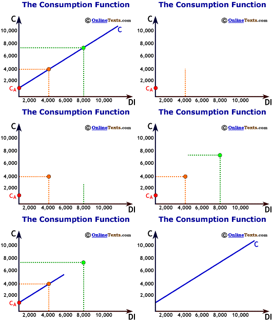
As the figure titled "The Consumption Function" illustrates, a consumption function shows the relationship between total consumer expenditures and total disposable income, holding all other determinants of consumption constant. No other factors are considered. The consumption function also assumes the relationship between consumption and disposable income is linear. The equation for the consumption function is:

C = C_A + MPC (DI)

The Marginal Propensity to Consume (MPC) tells us how much of an additional dollar of disposable income will be spent. For example, if the MPC = 0.80, then $0.80 of the next dollar earned will be spent. The MPC for an economy always lies between zero and one, 0 < MPC < 1.

Suppose the consumption function for the economy is the following:

C = 800 + 0.80 (DI), and DI = $6,000.

From this we know that C_A = 800, the MPC = 0.80, and total consumption is,
C = $800 + 0.80 * ($6,000) = $5,600.

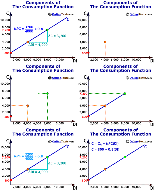
Two more points about the consumption function: First, as we have already stated above, the point at which the consumption function crosses the vertical axis is the level of Ca, autonomous consumption. In the figure titled "Components of the Consumption Function", the value for C_A is $800.

Second, the slope of the chart is the rise/run, or the change in C divided by the change in DI. Notice that this is exactly the same thing as the MPC. Therefore, the slope of the consumption is equal to the MPC. The slope of the line in the same figure is 0.80.

The Marginal Propensity to Save (MPS) is the complement to the Marginal Propensity to Consume. The MPS is defined as the change in saving divided by the change in disposable income. Since all Disposable Income is either consumed or saved, then the portion of additional disposable income not consumed must be saved. Therefore,

MPC + MPS = 1, or

MPS = 1 - MPC.

Determining Investment in the Income-Expenditure Model

Investment is the most volatile component of GDP. It accounts for approximately 17% of GDP. Investment is determined by interest rates, business confidence, taxes, and capacity utilization.

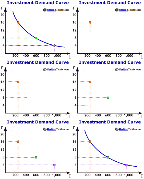
If interest rates rise, other things equal, investment falls. Why? Investment typically requires large amounts of upfront expenditures. Businesses must either borrow the resources externally or divert resources internally to the investment project. The costs of borrowing these funds is the interest rate. When interest rates are high, it is more expensive to borrow funds, so less investment is demanded. When interest rates are low, it is cheaper to borrow funds so more investment is demanded. The figure titled "Investment Demand Curve" plots the interest rate on the vertical axis and the quantity of investment on the horizontal axis. It is downward-sloping.

Taxes also impact investment. The return on investment depends on how heavily investment income is taxed (for example, the capital gains tax). Other things equal, higher taxes result in lower investment.

Capacity Utilization is the percentage of the existing plant and equipment that is being utilized. If capacity utilization rates are low, then the existing plant has room to expand and investment in the future will be lower. Conversely, if the utilization rates are high, then a firm might have to invest immediately to accommodate future growth.

In our simplified model, we assume that interest rates are already determined, and we assume that all other determinants of investment (such as business confidence) remain unchanged. Given a particular interest rate, we can determine the level of investment that will take place in the economy.

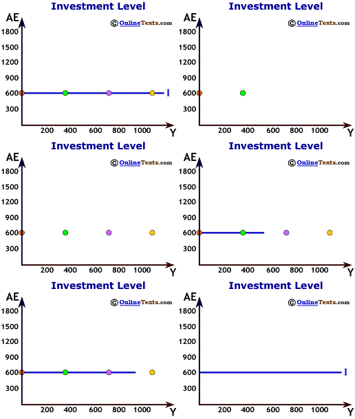
For example, suppose that the interest rate is 8.0 percent, and that rate corresponds to $600 of investment. We plot the level of investment in the figure titled "Investment Level." Aggregate expenditures go on the vertical axis while the level of income or GDP (Y) goes on the horizontal axis. The investment line is simply a horizontal line at $600. It has a slope of zero because we assume that investment does not vary with the level of income in the economy.

Aggregate Expenditures in the Income-Expenditure Diagram

If there are no taxes (which we assumed above), then disposable income (DI) and national income (Y) are equal to one another. So we can write:

C = C_A + MPC (DI) = C_A + MPC (Y), and
I = I_A,

where I_A is autonomous investment, or the level of investment independent of the level of income. We sum the two together to calculate Aggregate Expenditures:

AE = C + I = C_A + MPC (Y) + I_A

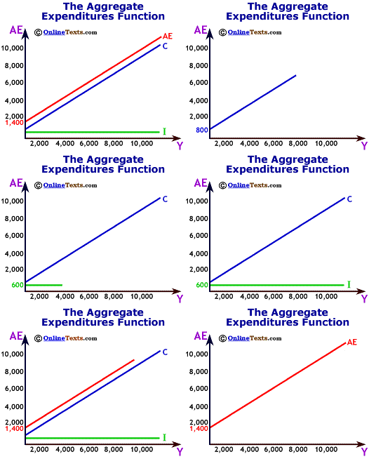
The level of Aggregate Expenditures depends upon the level of national income. As Y rises, so does AE. Therefore the Aggregate Expenditure schedule slopes upwards.

Notice that when Y=0, AE = 800 + 0.8(0) + 600 = 1400. But when Y = 100, AE = 800 + 0.8(100) + 600 = 1480. On the chart, the Aggregate Expenditure schedule is simply the vertical summation of the consumption function and the investment schedule at each level of output.

Equilibrium in the Income-Expenditure Model

As we saw from the Aggregate Demand/Aggregate Supply model, equilibrium is the point where the quantity produced (Y) is equal to the quantity demanded (AE), or
Y = AE.

The 45 degree line

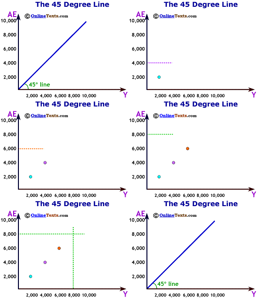
We employ a simple tool to help us find the equilibrium in the income-expenditure diagram. On any chart, if the horizontal and vertical axes have the same scale, then any (x,y) point on the 45 degree line will have the same value on both axes. In the figure titled "The 45 Degree Line," notice that every point on the 45 degree line has the same x and y value.

Every point on the 45 degree line is a point that satisfies the condition Y = AE. Therefore, we must look for equilibrium where the AE line crosses the 45 degree line.

Bringing it all together

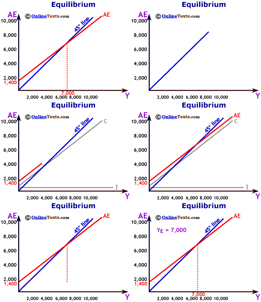
The figure titled "Equilibrium" puts all the elements together to determine the equilibrium level of income and Aggregate Expenditures in the economy. Notice that the AE line crosses the 45 degree line at $7,000. This is the only point on the chart where output (Y) is equal to expenditures (AE). Thus, the equilibrium level of output is $7,000.

If income (Y) were less than $7,000, say $6,000, then Aggregate Expenditures would exceed income, demand would be greater than output, and inventories would begin unexpectedly to shrink. If income (Y) were greater than $7,000, then Aggregate Expenditures would be less than output, and unwanted inventories would build. Only at $7,000 does production of final goods and services equal demand for final goods and services.

The Algebra of the Income-Expenditure Model

Recall that the equilibrium occurs when Y = AE. Since AE = C + I, then the equilibrium condition reduces to
Y = C + I.
And since
C = C_A + MPC(Y), and
I = I_A, then
Y = C_A + MPC(Y) + I_A.

We wish to solve for Y, but we must get all the Y's on the left-hand side. To do so, we subtract MPC(Y) from both sides, and we get
Y - MPC(Y) = C_A + I_A.

We distribute the Y term this way:
(1 - MPC)Y = C_A + I_A,
and then we divide both sides by (1 - MPC) to obtain
Y = (C_A + I_A)/(1 - MPC)

In our example above, we had the following equations:
C = 800 + 0.8 (Y), and
I = 600, so
Y = 800 + 0.8 (Y) + 600
Y - 0.8(Y) = 1400
(1- 0.8)Y = 1400
Y = 1400/(1 - 0.8)
Y = 1400/(0.2)
Y = 7,000

Once you get the hang of the algebra, you will see that this approach is much simpler and faster than charting the AE schedule and the 45 degree line. Fill in values for the MPC, C_A and I_A below to calculate the equilibrium level of income. Work out your own solution before you calculate your answer here.

Interactive Algebra Examples

Changes in Equilibrium Income

The Great Depression was a time when the economy was well below its full-employment level of output. But the economy seemed to be stuck at that low level with little chance of correcting itself. Economic history has shown us that, ironically, it was WWII that helped pull the economy out of recession. This doesn't mean that war is good--indeed most people would rather have lived in economic depression than have their sons and daughters die in such a horrible war--yet the war did have expansionary effects on the economy. Massive demand for military goods and services shifted the Aggregate Expenditure curve upward and increased the equilibrium level of income. The unemployment rate fell from a peak of 25 percent in the early 1930s to under 2 percent in the early 1940s! Let's take a closer look at the income-expenditure model to see what was going on. We do not introduce government expenditures into the model at this point (see Chapter 12), but we do look at the impact of higher investment spending.

Changes in Autonomous Investment

One positive benefit from World War II was that autonomous investment increased. Demand for war goods and services increased investment as soldiers needed food, clothing, and weapons. Investment also increased as factories such as General Motors switched from producing cars to producing tanks.

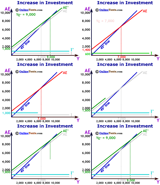
In the income-expenditure model, this increase in autonomous investment shifted the AE schedule upward and led to an increase in equilibrium income. The increased production and expenditures lowered unemployment and stimulated the domestic economy.

In the figure titled "Increase in Investment" we assume that Investment increases from $600 to $1,000. The Aggregate Expenditures curve shifts by the same vertical distance as the shift in investment. Equilibrium output increases from $7,000 to $9,000.

As a general rule, any increase in autonomous consumption or investment shifts the AE schedule upwards and leads to a rise in equilibrium income. The opposite occurs when autonomous consumption or autonomous investment declines. In the interactive table above, experiment with increasing and decreasing the values of C_A and I_A and see what happens to equilibrium income. If autonomous consumption increases from $800 to $900, does the equilibrium level of income rise by $100 or by more than $100? Why?