Chapter Twelve: Lecture Notes -- Fiscal Policy


Stabilization policy is an attempt to dampen the fluctuations in the economy's level of output through time to achieve low inflation and low unemployment.

The government's attempt to stabilize the economy is know as fiscal policy.
Stabilization policy is an attempt to dampen the fluctuations in the economy's level of output through time to achieve low inflation and low unemployment. The two U.S. organizations which conduct stabilization policy on a large scale are the government and the Federal Reserve. The government's attempt to stabilize the economy is know as fiscal policy (which we deal with here), while the Federal Reserve's attempt at stabilization is called monetary policy, which we deal with in Chapter 15.

Fiscal policy is the attempt by the government to deliberately manipulate its budget position with a goal of stabilizing prices, promoting growth, and minimizing unemployment. The role of the federal government in the U.S. economy has increased substantially since the Great Depression and many people perceive that the government is responsible for providing significant economic assistance in times of recession. This chapter explores exactly what fiscal policy is and how it is implemented. We also look at a particular branch of fiscal policy that rides various waves of popularity called Supply-Side Economics.


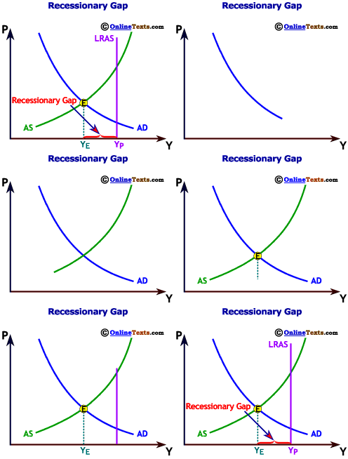
A recessionary gap occurs when actual output is less than potential output.


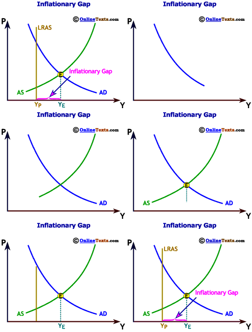
An inflationary gap occurs when equilibrium output exceeds potential output.

Recessionary and Inflationary Gaps

Recall from the Aggregate Demand/Aggregate Supply model of Chapter 8 that an economy can be at a short-run equilibrium even if labor resources are not fully utilized. In addition, the economy may be in equilibrium at a point where labor resources are more than fully employed. Given these scenarios, there may be room for the government to intervene in the economy to push the economy to a new equilibrium closer to full employment. We explore two such scenarios called recessionary and inflationary gaps.

Recessionary Gaps

Recessionary Gap - Equilibrium Output is Less than Potential Output

A recessionary gap occurs when actual equilibrium output (YE) is less than potential output (YP), or YE < YP. The amount of the recessionary gap is the difference between potential and actual output. In this case, the economy has an unemployment rate above the natural rate of unemployment. In the figure titled "Recessionary Gap," the short-run equilibrium occurs at the intersection of Aggregate Demand and Aggregate Supply at YE. Because the economy is below potential output, there is room for fiscal policy to boost the economy to its full employment level.


Inflationary Gaps

Inflationary Gap - Equilibrium Output is Greater than Potential Output

An inflationary gap occurs when equilibrium output exceeds potential output, or YE > YP. The amount of the inflationary gap, as illustrated in the figure titled "Inflationary Gap" is the horizontal difference between actual and potential output. In this case, the unemployment rate is below the natural rate, which puts upward pressure on wages and, hence, prices. Again, there is room for fiscal policy to slow the economy to reduce the inflationary pressure.


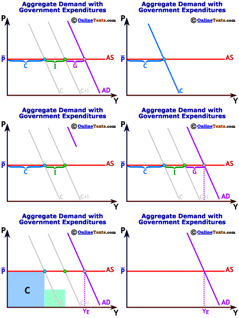
Equilibrium output with government expenditures included as a component of Aggregate Demand is Y = C + I + G.

Adding Government to the Fixed-Price Model

Government Expenditures are a Component of AD

To understand better the implications of adding the government sector to the Aggregate Demand/Aggregate Supply model, we employ the fixed-price model developed in Chapter 10. The Aggregate Demand/Aggregate Supply model with an upward-sloping Aggregate Supply curve could be used as well, but the multiplier effects would be smaller.

Equilibrium output in the fixed-price model without government expenditures was simply Y = C + I. With inclusion of G in the model, equilibrium output is now Y = C + I + G. Adding G to the equation simply shifts the Aggregate Demand curve to the right. Note that with a flat Aggregate Supply curve, the price level does not change when government expenditures are added to Aggregate Demand. For example, if consumption is $5,000, investment is $2,000 and government expenditures are $3,000, then equilibrium output is $10,000. The figure titled "Aggregate Demand with Government Expenditures" illustrates that, given the price level, the three components of Aggregate Demand sum to the equilibrium level of output YE.


The government has three tools to conduct fiscal policy which include a change in the level of government expenditures, a change in taxes, and a change in transfer payments.


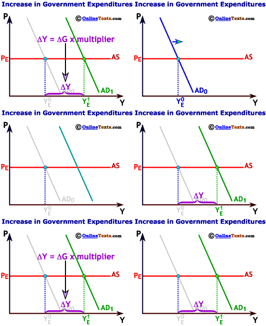
By increasing government expenditures, the government shifts the Aggregate Demand curve to the right.

Tools of Fiscal Policy

The government has three "tools" to conduct fiscal policy:

  1. change in the level of government expenditures,
  2. change in taxes, and
  3. change in transfer payments.
We discuss each in turn.

Tool #1: Change in Government Expenditures

Increased Government Expenditure Shifts out the AD Curve

The government purchases billions of dollars of goods and services each year. By changing the total amount that it purchases, the government can change Aggregate Demand. As the figure titled "Increase in Government Expenditures" illustrates, an increase in government expenditures--like any autonomous component of Aggregate Demand--shifts the Aggregate Demand curve to the right (from AD0 to AD1), which leads to the usual multiplier effects. So in the fixed price model with a simple output multiplier, a $1 change in G ultimately increases Y by 1/(1-MPC) × change in G.

For example, suppose that the economy is in a recessionary gap of $800, and the marginal propensity to consume (MPC) in the economy is 0.75. How much should government expenditures be changed in order to eliminate the recessionary gap? The answer is not $800, but $200 because the multiplier in this example is 4. The increase in government expenditures will induce more consumption spending as incomes rise.

After the terrorist attacks in the U.S. on September 11, 2001, the government responded by increasing defense-related output. Additional terrorism agents were hired and trained, the government took over airport security, military reservists went from part-time duty to full-time duty, and so on. These expenditures increased Aggregate Demand and generated corresponding multiplier effects.
Conversely, a decrease in government expenditures shifts the Aggregate Demand curve to the left, which leads to a decline in output. Remember that multiplier effects come into play in this case as well, only in the reverse direction.


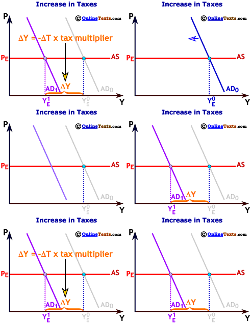
By increasing taxes the government shifts the Aggregate Demand curve to the left.


The tax multiplier is given by the formula -MPC/(1-MPC).
Tool #2: Change in Taxes

Increase in Taxes Reduces Shifts the AD Curve Back

The government sets tax policy, which determines how much of the nation's gross income will be taxed. The U.S. income tax is a proportional tax in that a percentage of each person's income is taxed. The total amount of tax each person pays depends on her income. When the government raises taxes, more of a person's gross income goes to the government so she has less disposable income for personal use. Less disposable income leads to less consumption. An increase in taxes, therefore, shifts the Aggregate Demand curve to the left. Such a scenario is illustrated in the figure titled "Increase in Taxes."

In June 2001 President Bush pushed a $1.3 trillion tax cut through Congress. The full tax reduction of $1.3 trillion will be realized over a ten-year period; nevertheless, the change in taxes shifts the Aggregate Demand curve to the right. Part of the tax change gave a rebate of up to $600 to households. Hence, personal income and consumption increased. Why would President Bush enact such a policy? His motives may have been complicated including a desire to be elected, but part of the reason was to stimulate the economy to prevent the nation from slipping into recession. In other words, the President and his advisors sensed that the nation was slipping into a recessionary gap and he wanted to enact policy to reduce the probability of a recession occurring.

With the advantage of hindsight, the timing of the tax cut was ideal, even if one questions the wisdom of the tax cuts as a whole. The economy officially slipped into recession in March 2001; the tax cuts gave consumers additional disposable income over the next few months. Indeed, strong consumer spending was the major reason that the recession was relatively mild.

The Tax Multiplier

Tax changes are also subject to the output multiplier effect, but the process is slightly more complicated than that for a change in government expenditures. Unlike a change in government expenditures, a change in the tax rate impacts Aggregate Demand indirectly by first reducing disposable income, which then reduces consumption. Recall that disposable income is equal to national income (Y) less taxes (T) plus transfer payments (TR), or DI = Y - T + TR. If taxes rise, disposable income falls. The decline in disposable income reduces consumption, but not by the full amount of the income decline. When taxes rise, disposable income falls by the MPC times the change in disposable income because only a portion of the lost income would have been consumed. Let's work through an example.

Suppose that Mitch has a consumption function of the following form:
C = $100 + 0.8(DI)
and his disposable income goes from $1,000 to $900 per month because his taxes increase by $100 per month. At $1,000 Mitch's monthly consumption was
C = $100 + 0.8($1,000) = $900,
but with disposable income at $900, his monthly consumption falls to
C = $100 + 0.8($1,000-$100) = $820.
Mitch's consumption declined by $80, which is equal to the MPC (0.8) times the change in taxes ($100).

Recall that the multiplier effect is given by the formula

For an increase in taxes, the initial decrease in Aggregate Demand is not the amount of the tax change, but the MPC times the tax change, or

Because we are ultimately interested in the relationship between a change in output and a change in taxes, we rewrite the above equation as:

where -MPC/(1-MPC) is the tax multiplier. For example, if the MPC is 0.8, then the tax multiplier is -0.8/(1-0.8) = - 4. Note that the tax multiplier is smaller and has the opposite sign as the simple output multiplier. The smaller size is because the effect of a tax increase on Aggregate Demand is indirect. The opposite sign is because an increase in taxes decreases output. Conversely, a decrease in taxes increases output.


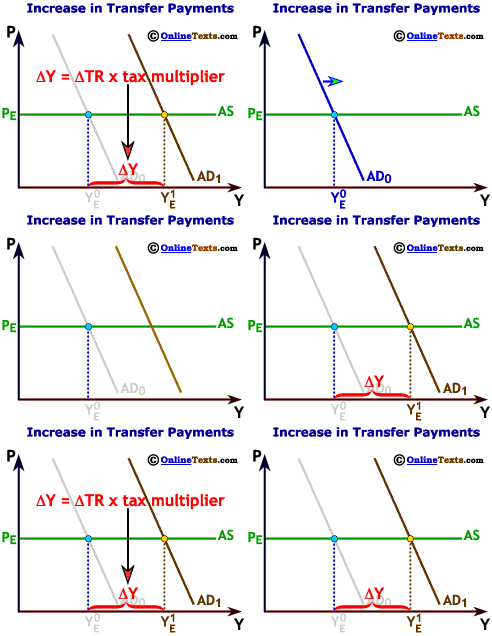
By increasing transfer payments the government can shift the Aggregate Demand curve to the right. The increase in output is equal to the tax multiplier times the change in transfer payments, but, unlike tax increases, output increases when transfer payments increase.
Tool #3: Change in Transfer Payments

An Increase in Transfer Payments Shifts Out AD

Transfer payments (TR) are distributions of income to individuals who do not directly work for the income. Examples are Social Security payments, welfare assistance, Medicare, farm assistance and food stamps. Transfer payments account for more than half of the U.S.$2 trillion annual federal budget. If the government increases transfer payments, disposable income rises, and thus consumption increases. As the figure titled "Increase in Transfer Payments" illustrates, if transfer payments are increased, the Aggregate Demand curve shifts to the right. Conversely, a decrease in transfer payments shifts the Aggregate Demand curve to the left.

A change in transfer payments also affects Aggregate Demand indirectly by first changing the level of disposable income. An increase in Social Security payments of $100 per month, for example, increases consumption spending by the MPC times the $100. The size of the transfer payment multiplier effect, therefore, is identical to that of a tax change. The direction of the transfer multiplier effect, however, is just the opposite of the effect of the tax multiplier effect. Whereas a $1 increase in taxes decreases equilibrium output by MPC/(1-MPC), a $1 increase in transfer payments increases equilibrium output by MPC/(1-MPC).


Expansionary and Contractionary Fiscal Policy

TABLE 1
Fiscal Policy
ExpansionaryContractionay
Increase GDecrease G
Decrease TIncrease T
Increase TRDecrease TR

The government can conduct either expansionary or contractionary policy depending on the desired outcome. Table 2 illustrates the government's options. If the economy is in a recessionary gap, the government will want to stimulate Aggregate Demand via expansionary fiscal policy. Expansionary policy is implemented via some combination of these three tools:

  • increase government expenditures,
  • decrease taxes, or
  • increase transfer payments.

If the economy is in an inflationary gap, the government will want to reduce Aggregate Demand via contractionary fiscal policy. Contractionary policy is implemented via some combination of these three tools:

  • decrease government expenditures,
  • increase taxes, or
  • decrease transfer payments.


Fiscal Policy with an upward-sloping AS Curve

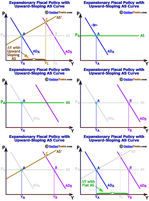
Fiscal Policy With Upward Sloping AS Curve If the Aggregate Supply curve is upward sloping rather than horizontal (as we assume in the fixed-price model), then two things are different about fiscal policy:
  1. An increase in government expenditures increases both output and the price level, as illustrated in the figure titled "Expansionary Fiscal Policy with Upward Sloping AS Curve."
  2. Output multiplier effects will be smaller because some of the impact will be felt in higher prices, decreasing Aggregate Demand. Rather than increasing from YA to YB, output only increases to YC.

The closer that the economy is to its potential output, the smaller the impact on output, and the larger the impact on prices.


Discretionary fiscal policy is a deliberate change in policy whereas automatic stabilizers adjust automatically to the needs of the economy.

Discretionary Fiscal Policy vs. Automatic Stabilizers

Discretionary Fiscal Policy

Discretionary Policy is policy that must be deliberately enacted by Congress and/or the President. For example, a change in laws impacting unemployment insurance, welfare, or tax rates qualify as discretionary fiscal policy. Inherent difficulties arise in conducting good discretionary fiscal policy. First, there are severe time lags. Lags result from any of these three sources:

  • Recognition lag: the time needed for legislators to recognize that policy needs to be changed due to a change in the business cycle.

  • Implementation lag: the time needed to change the policy. Because of partisan politics, this lag can be considerable. Decisions on taxes, transfer payments, and government spending are usually made with more concern for politics than for economics.

  • Impact lag: the time elapsed between the implementation of the changed policy and its impact on the economy. It is possible that by the time deliberate fiscal policy is enacted and impacts the economy, the reason for the action has already passed. The average recession lasts for 11 months. It is possible that the lag time for fiscal policy is longer than 11 months.

A second difficulty is that the growth in the budget deficit has made discretionary fiscal policy less of an option. Deliberate increases in government spending are not popular because they increase the budget deficit. Although this concern has diminished since the late 1990s, the fear of a return to high deficits may be enough to dampen the effectiveness of fiscal policy.

Automatic Stabilizers

Automatic stabilizers are policies that increase government outlays and decrease taxes automatically during recessions, and reduce government outlays and increase taxes automatically during inflationary periods. No deliberate government action is required. Examples are welfare payments, unemployment insurance, and proportional income taxes. Automatic stabilizers automatically dampen the business cycle. When the economy goes into recession, spending on poverty programs and other transfer programs increase while tax revenues decrease. These policies are free from recognition and implementation lags, and they are also free from politics. Partially because of automatic stabilizers, budget deficits increase during recessions and decrease in times of growth and recovery.


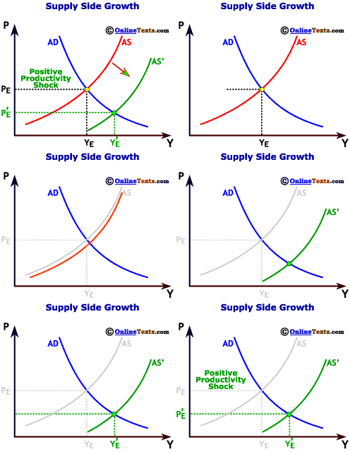
Supply-side economics wishes to conduct policy with the goal of shifting the Aggregate Supply curve to the right.

Supply-Side Economics: Introduction

Supply Side Policies Attempt to Shift Out the AS Curve

Supply-side economics is a school of thought that challenges the emphasis of Keynesian economics on the demand side of the economy. As the figure titled "Supply Side Growth" illustrates, supply-siders wish to increase economic growth and spur the economy by stimulating the supply side of the economy. In its simplest form, supply-side economics wishes to conduct policy with the goal of shifting the Aggregate Supply curve to the right. Such a policy leads to higher output and a lower price level (or in the real world, lower rates of inflation). The outcome seems to be the best of both possible worlds: a world of high employment and low inflation.


Supply-side economics has a colorful but controversial history in the United States. President Kennedy first advocated and enacted a modest supply-side policy in the early 1960s. President Reagan followed suit in the early 1980s with a much more substantial policy change. In a run for the 1996 Presidency, Senator Dole advocated supply-side policies to stimulate the economy. The theory of supply-side economics is not all that controversial, but the implementation and impact of supply side economics are vigorously contested. Here we examine the main propositions of these policies.


By decreasing taxes the government releases resource constraints on the economy, which spurs capital formation and labor input.

Unleashing Labor and Capital Resources

One of the supply-side themes is that government regulations and high taxes constrain the growth of the supply-side of the economy. Production comes form combining labor and capital with a level of technology. If income taxes are too high, for example, many people may choose not to work in the market. It is not worth the opportunity cost of the time spent at work if say, 50 cents on every dollar goes towards taxes. By reducing taxes, more labor will be attracted to the market thus shifting the Aggregate Supply curve to the right.

A similar argument holds for capital formation. Excess regulations and taxes diminish the incentives for saving and investment. By lowering the tax rates and simplifying regulations, incentives for investment increase and more capital formation occurs. The increased level of capital in the economy shifts the Aggregate Supply curve to the right.


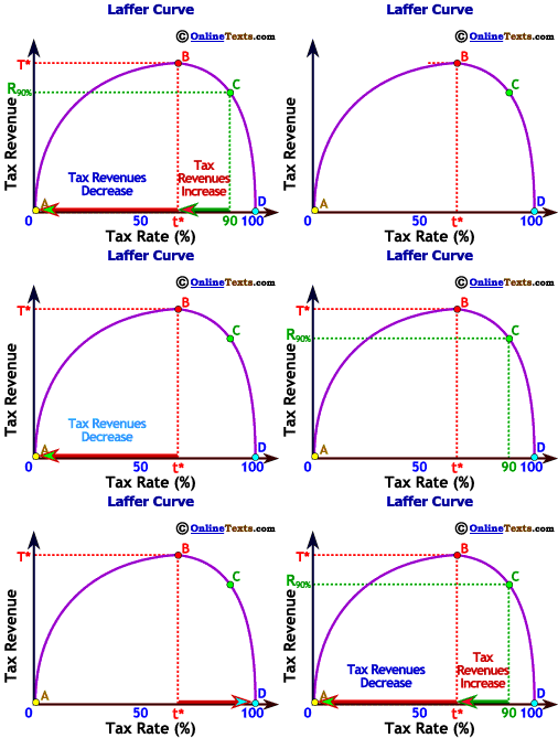
The Laffer curve shows that a decrease in tax rates may actually lead to higher tax revenues.

The Laffer Curve

What about the budget deficit? The reduction in taxes means that the tax revenue raised to finance government spending is diminished. With the same amount of government expenditures, the deficit must increase. One could even argue that the larger deficits crowd out private investment and slow economic growth, limiting or possibly reversing the goal of supply-side policies. There are two responses to this objection. First, supply-side policies typically advocate a smaller role for the government; they recommend a reduction in government spending to offset the lower tax revenues.

The second response is that cutting tax rates does not necessarily lead to lower tax revenues. How can this be? If the tax reductions stimulate enough growth in GDP by increases in labor and capital supply, then the tax base for the economy increases over time. Tax revenues, therefore, may actually increase. A rise in short-term deficits is likely, but over the longer term the economy's growth will more than offset the decline caused by lower tax rates. The theory was popularized by economist Arthur Laffer and the graphical representation, termed the "Laffer Curve," is plotted in the figure titled "Laffer Curve." The Laffer Curve

Four points on the curve are labeled, points A through D. Point A lies at the origin because a zero tax rate produces zero tax revenue for the government. Point D is at the 100 percent tax rate, which also produces zero tax revenue because if income were taxed at a 100 percent level, people would have no incentive to produce anything at all. All income would be taken by the government. Point B shows the tax rate (t*) in the economy that maximizes tax revenue (T*). In this chart it is arbitrarily drawn at around 70 percent but it could be lower or higher. The important concept is that if the economy is to the right of point B such as point C, a decrease in the tax rate actually increases tax revenues because the increase in taxes from new output and income offsets the tax losses from the lower tax rate. On the other hand, if the economy is to the left of point B, a decrease in the tax rate decreases tax revenues and leads to larger budget deficits.

Where was the economy at in the early 1980s? After the enactment of the Reagan tax cuts, budget deficits increased to record levels and remained high through the mid-1990s. Granted, not all of the high deficits resulted form the tax cuts. Nevertheless, this evidence suggests--as most economists suspected--that the economy was to the left of point B when the tax cuts were enacted.


Many Keynesian economists argue that the impact on the supply side of the economy is minor.

Is There Consensus?

Most economists do not argue about the theory of supply-side economics. It is agreed that lower tax rates and less regulation will stimulate labor and capital formation. The argument is primarily about the size of these impacts. Many Keynesian economists argue that the impact on the supply side of the economy is minor. The economy may grow slightly faster, but it is not nearly enough to offset the loss of tax revenues.

Moreover, much of the controversy over supply-side policies results from differences in societal values. Advocates of supply-side economics typically wish to see government programs and regulations reduced. They also wish to see income taxes for the poor and the wealthy reduced. Opponents argue that supply-siders wish to cut taxes for the wealthy at the expense of important social programs. Supply-side advocates tend to be Republican in political alliance; many Democrats oppose supply-side policies for the same reasons that they oppose the platform of the Republican party. So much of the debate comes down to differences over the proper role of government in our lives.

Perhaps the common belief is that the Reagan tax cuts and fiscal policies in the 1980s increased economic growth, reduced the non-defense portion of government spending, and increased budget deficits. The debate is over whether or not these changes were "good" for the economy and society.


Useful Web Resources


Copyright © 1995-2006 OnlineTexts.com - All Rights Reserved