Chapter Three: Notes -- Supply and Demand


Why do teachers earn $30,000 per year while some professional athletes earn $18 million per year? Isn't education more important than sports? Why is the price of an ounce of diamonds far higher than the price of an ounce of water? People need water to survive; diamonds are luxuries. These types of paradoxes abound. As you may have guessed by now, the answers lie in the forces of supply and demand.

Have you ever awakened at 3am with a bad headache and had to rush to the pharmacy to buy some aspirin? How did the store know to have aspirin in stock? You certainly didn't phone ahead or even plan on buying the aspirin--certainly not at 3am. How much aspirin do you think consumers purchase each year in the United States? Who coordinates this production to make sure there is enough? What price should be charged for aspirin? In socialist economies, government officials ultimately decide how much aspirin to produce per year and they also decide what price to charge. If the government officials do not plan for your headache at 3am, you are out of luck. In fact, shortages and lack of product selection are commonplace in socialist economies.

The amazing thing about a capitalist system is that there is no central planner. Government officials don't tell businesses how much aspirin to produce nor the price to charge. Private producers figure out production levels and prices on their own. The consumer indirectly tells the producer what she is willing to buy and how much she is willing to pay based on her actual spending patterns. The producer supplies the product if she can make a profit by doing so. The forces of supply and demand coordinate all this activity.

Suppose consumers decide they do not like small fuel-efficient cars anymore. They prefer the larger four-wheel drive sub-utility vehicles. Who tells the auto producers to change their production? You guessed it--the forces of supply and demand hold the answer. Producers see that the smaller cars are sitting on their lots not selling (demand declines) while the large vehicles are selling like hot cakes (demand increases). The producers respond to the changing consumer tastes by discounting the smaller cars and producing more of the larger ones.

Supply and demand analysis is an extremely powerful analytical tool, yet it is little understood and often confused. We begin by noting that there is no "law of supply and demand." There are two separate laws: a law of supply and a law of demand. Each works independently of the other. We first discuss the law of demand, then the law of supply, and see how the laws interact to determine prices and quantities.
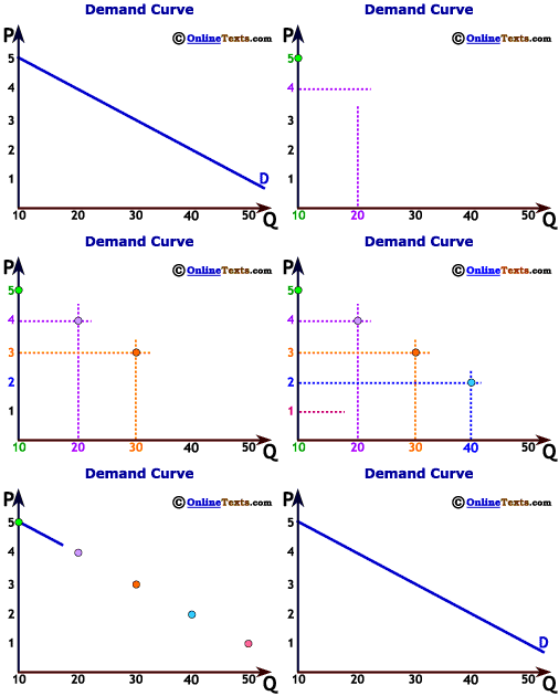


The law of demand holds that other things equal, as the price of a good or service rises, its quantity demanded falls.


A demand curve is a graphical depiction of the law of demand, plotting price on the vertical axis and quantity demanded on the horizontal axis.

The Law of Demand and the Demand Curve

We begin with demand because demand is usually easier to understand from our personal experiences. We are all consumers and we all demand goods and services. Demand is derived from consumers' tastes and preferences, and it is bound by income. In other words, given a limited income (whether it be $30,000 or $5 million), the consumer must decide what goods and services to purchase. Within his budget, the consumer will purchase those goods and services that he likes best. Each consumer will purchase different things because individual preferences and incomes differ.

The law of demand holds that other things equal, as the price of a good or service rises, its quantity demanded falls. The reverse is also true: as the price of a good or service falls, its quantity demanded increases. This law is a simple, common sense principle. Think of your trips to the grocery store. When the price of orange juice rises, for example, you buy less of it. When that item is on sale, you purchase more of it. This is all that we mean by the law of demand.

Table 1 lists the monthly quantity of rental videos demanded by an individual given several different prices. If the rental price is $5, the consumer rents 10 videos per month. If the price falls to $4, the quantity demanded increases to 20 videos, and so on. The figure titled "Demand Curve" plots the inverse relationship between price and quantity demanded.

TABLE 1
Demand for Videos
PriceQuantity Demanded
$510
$420
$330
$240
$150
Demand is downward sloping because desired quantity demanded falls when price increases

A demand curve is a graphical depiction of the law of demand. We plot price on the vertical axis and quantity demanded on the horizontal axis. As the figure illustrates, the demand curve has a negative slope, consistent with the law of demand.


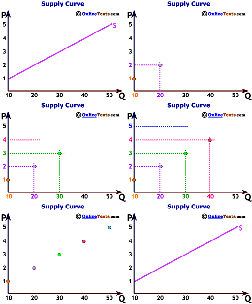
The law of supply holds that other things equal, as the price of a good rises, its quantity supplied will rise.


A supply curve is a graphical depiction of a supply schedule plotting price on the vertical axis and quantity supplied on the horizontal axis.

The Law of Supply and the Supply Curve

Supply is slightly more difficult to understand because most of us have little direct experience on the supply side of the market. Supply is derived from a producer's desire to maximize profits. When the price of a product rises, the supplier has an incentive to increase production because he can justify higher costs to produce the product, increasing the potential to earn larger profits. Profit is the difference between revenues and costs. If the producer can raise the price and sell the same number of goods while holding costs constant, then profits increase.

The law of supply holds that other things equal, as the price of a good rises, its quantity supplied will rise, and vice versa. Table 2 lists the quantity supplied of rental videos for various prices. At $5, the producer has an incentive to supply 50 videos. If the price falls to $4 quantity supplied falls to 40, and so on. The figure titled "Supply Curve" plots this positive relationship between price and quantity supplied.

TABLE 2
Supply of Videos
PriceQuantity Supplied
$550
$440
$330
$220
$110
Supply is upward sloping because desired quantity supplied increases with price

A supply curve is a graphical depiction of a supply schedule plotting price on the vertical axis and quantity supplied on the horizontal axis. The supply curve is upward-sloping, reflecting the law of supply.


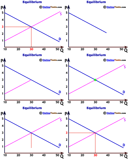
Equilibrium occurs at the price in which quantity demanded equals quantity supplied.


A shortage occurs when quantity demanded exceeds quantity supplied.


A surplus occurs when quantity supplied exceeds quantity demanded.

Equilibrium: Determination of Price and Quantity

What price should the seller set and how many videos will be rented per month? The seller could legally set any price she wished; however, market forces penalize her for making poor choices. Suppose, for example, that the seller prices each video at $20. Odds are good that few videos will be rented. On the other hand, the seller may set a price of $1 per video. Consumers will certainly rent more videos with this low price, so much so that the store is likely to run out of videos. Through trial and error or good judgement, the store owner will eventually settle on a price that equates the forces of supply and demand.

In economics, an equilibrium is a situation in which:

  • there is no inherent tendency to change,
  • quantity demanded equals quantity supplied, and
  • the market just clears.
At the market equilibrium, every consumer who wishes to purchase the product at the market price is able to do so, and the supplier is not left with any unwanted inventory. As Table 3 and the figure titled "Equilibrium" demonstrate, equilibrium in the video example occurs at a price of $3 and a quantity of 30 videos.

At the equilibrium price desired quantity demanded and supplied are equal
TABLE 3
Video Market Equilibrium
PriceQuantity
Demanded
Quantity
Supplied
$51050
$42040
$33030
$24020
$15010


Suppose that the video store owner charges $2 per video rental. The result is a shortage. A shortage occurs when quantity demanded exceeds quantity supplied. At a price of $2, quantity supplied is 20 videos but quantity demanded is 40 videos. Some consumers who wish to rent videos are unable to do so. A shortage implies the market price is too low. Shortages are common in socialist economies because low prices for common staples such as food and energy are set by the government. Rather than pay higher prices, people are forced to wait in long lines to purchase the desired goods and services.

A surplus occurs when quantity supplied exceeds quantity demanded. With a rental price of $4, quantity supplied is 40 videos but quantity demanded is only 20 videos. A surplus of 20 videos exists. A surplus implies the market price is too high.

Perhaps more often than not, markets are not exactly in equilibrium. Minor surpluses and shortages are common in a market economy. A stroll through most malls at the end of the clothing season reveals the excess clothing inventory that many stores carry. How do they manage this situation? By lowering prices. Lower prices reduce the incentive for stores to carry the clothes while simultaneously increasing the incentive for consumers to purchase the clothes. The important point is that even though a market may not be in perfect equilibrium, it tends to gravitate towards equilibrium over time. This fact makes markets stable most of the time such that persistent surpluses and shortages are uncommon and self-correcting.

Persistent and severe shortages and surpluses do occur in the U.S. economy every now and then. At the end of 1998, for example, the supply of hogs in the U.S. markets was so much greater than demand that the price of hogs fell from about $50 per hundredweight to $13 per hundredweight. Many farmers were so badly hurt by that experience that they left the hog market completely--a painful but self-correcting force. In the late 1970s the relative shortage of gasoline resulted in long lines at the gas pumps. The shortages lasted for a couple years until oil producers stepped up production and consumers learned to use fuel more efficiently.


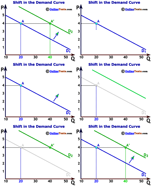
It is essential to distinguish between a movement along a demand curve and a shift in the demand curve.

A Shift versus a Movement Along a Demand Curve

The demand curve shifts due to changes in factors other than price

It is essential to distinguish between a movement along a demand curve and a shift in the demand curve. A change in price results in a movement along a fixed demand curve. This is also referred to as a change in quantity demanded. For example, an increase in video rental prices from $3 to $4 reduces quantity demanded from 30 units to 20 units. This price change results in a movement along a given demand curve. A change in any other variable that influences quantity demanded produces a shift in the demand curve or a change in demand. The terminology is subtle but extremely important. The majority of the confusion that students have with supply and demand concepts involves understanding the differences between shifts and movements along curves.

TABLE 4
Change in Demand for
Videos after Incomes Rise
PriceInitial Quantity
Demanded
New Quantity
Demanded
Quantity
Supplied
$5103050
$4204040
$3305030
$2406020
$1507010

Suppose that incomes in a community rise because a factory is able to give employees overtime pay. The higher incomes prompt people to rent more videos. For the same rental price, quantity demanded is now higher than before. Table 4 and the figure titled "Shift in the Demand Curve" represent that scenario. As incomes rise, the quantity demanded for videos priced at $4 goes from 20 (point A) to 40 (point A'). Similarly, the quantity demanded for videos priced at $3 rises from 30 to 50. The entire demand curve shifts to the right.

When the demand curve shifts the market moves to a new equilibrium

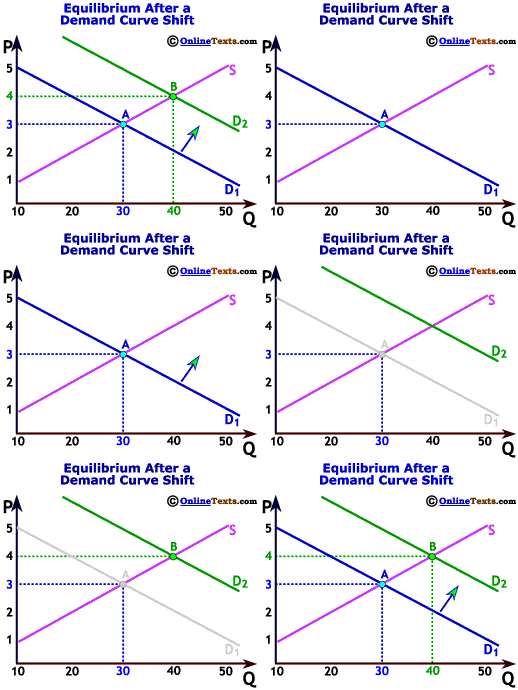
A shift in the demand curve changes the equilibrium position. As illustrated in the figure titled "Equilibrium After a Demand Curve Shift" the shift in the demand curve moves the market equilibrium from point A to point B, resulting in a higher price (from $3 to $4) and higher quantity (from 30 to 40 units). Note that if the demand curve shifted to the left, both the equilibrium price and quantity would decline.


Substitutes are goods that can be consumed in place of one another. Complements are goods that are normally consumed together

Factors that Shift the Demand Curve

We list and explain four factors that can shift a demand curve:

  1. Change in consumer incomes: As the previous video rental example demonstrated, an increase in income shifts the demand curve to the right. Because a consumer's demand for goods and services is constrained by income, higher income levels relax somewhat that constraint, allowing the consumer to purchase more products. Correspondingly, a decrease in income shifts the demand curve to the left. When the economy enters a recession and more people become unemployed, the demand for many goods and services shifts to the left.

  2. Population change: An increase in population shifts the demand curve to the right. Imagine a college town bookstore in which most students return home for the summer. Demand for books shifts to the left while the students are away. When they return, however, demand for books increases even if the prices are unchanged. As another example, many communities are experiencing "urban sprawl" where the metropolitan boundaries are pushed ever wider by new housing developments. Demand for gasoline in these new communities increases with population. Alternatively, demand for gasoline falls in areas with declining populations.

  3. Consumer preferences: If the preference for a particular good increases, the demand curve for that good shifts to the right. Fads provide excellent examples of changing consumer preferences. Each Christmas season some new toy catches the fancy of kids, and parents scramble to purchase the product before it is sold out. A few years ago, "Tickle Me Elmo" dolls were the rage. In the year 2000 the toy of choice was a scooter. For a given price of a scooter, the demand curve shifts to the right as more consumers decide that they wish to purchase that product for their children. Of course, demand curves can shift leftward just as quickly. When fads end suppliers often find themselves with a glut of merchandise that they discount heavily to sell.

  4. Prices of related goods: If prices of related goods change, the demand curve for the original good can change as well. Related goods can either be substitutes or complements.
    • Substitutes are goods that can be consumed in place of one another. If the price of a substitute increases, the demand curve for the original good shifts to the right. For example, if the price of Pepsi rises, the demand curve for Coke shifts to the right. Conversely, if the price of a substitute decreases, the demand curve for the original good shifts to the left. Given that chicken and fish are substitutes, if the price of fish falls, the demand curve for chicken shifts to the left.
    • Complements are goods that are normally consumed together. Hamburgers and french fries are complements. If the price of a complement increases, the demand curve for the original good shifts to the left. For example, if McDonalds raises the price of its Big Mac, the demand for french fries shifts to the left because fewer people walk in the door to buy the Big Mac. In contrast, If the price of a complement decreases, the demand curve for the original good shifts to the right. If, for example, the price of computers falls, then the demand curve for computer software shifts to the right.


Like demand curves, it is essential to distinguish between a movement along a given supply curve and a shift in a supply curve.

A Shift versus a Movement Along a Supply Curve

A shift in supply is the result of a change other than market price

As with demand curves, it is essential to distinguish between a movement along a given supply curve and a shift in a supply curve. A change in price results in a movement along a fixed supply curve. This is also referred to as a change in quantity supplied. For example, if the rental price of videos rises from $3 to $4, quantity supplied increases from 30 to 40 units. A change in any other variable that influences quantity supplied produces a shift in the supply curve or a change in supply.

TABLE 5
Change in Supply due to an
Increase in Video Costs
PriceQuantity
Demanded
Initial Quantity
Supplied
New Quantity
Supplied
$5105030
$4204020
$3303010
$240200
$150100

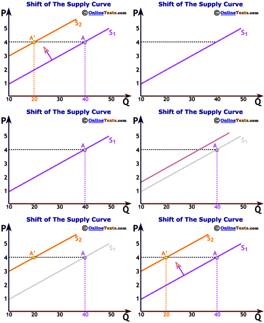
Suppose for example that the video store purchases its videos from Hollywood Inc. but Hollywood Inc. just increased its prices. Now the video rental store has to pay more to purchase the videos that it makes available to customers. For a given rental price of videos, the video store has to reduce the quantity of videos it supplies. For the same price, quantity supplied will be lower than before. Table 5 and the figure titled "Shift in the Supply Curve" show this scenario. Initially at a price of $4, quantity supplied was 40 (point A). After the leftward shift of the supply curve, at the same price of $4, quantity supplied is only 20 units (point A').

A shift in supply leads to a new equilibrium

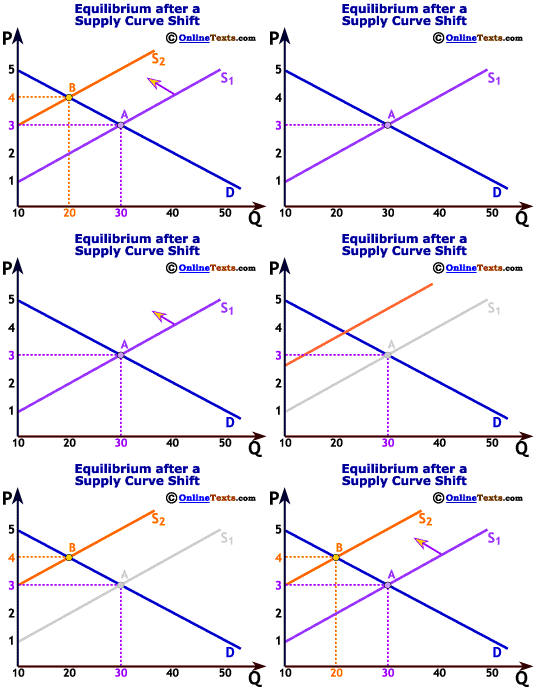
Equilibrium price and quantity change after a shift in the supply curve. The figure titled "Equilibrium After a Supply Curve Shift" plots the new equilibrium after the leftward shift of the supply curve. The equilibrium moves from point A to point B, resulting in a higher price (from $3 to $4) and lower quantity (from 30 to 20). Conversely, a rightward shift of the supply curve reduces the equilibrium price and increases the equilibrium quantity.


An increase in technology shifts the supply curve to the right.

Factors that Shift the Supply Curve

We list and explain three factors that shift a supply curve:
  1. Change in input costs: An increase in input costs shifts the supply curve to the left. A supplier combines raw materials, capital, and labor to produce the output. If a furniture maker has to pay more for lumber, then her profits decline, all else equal. The less attractive profit opportunities force the producer to cut output. Alternatively, car manufacturer may have to pay higher labor costs. The higher labor input costs reduces profits, all else equal. For a given price of a car, the manufacturer may trim output, shifting the supply curve to the left. Conversely, if input costs decline, firms respond by increasing output. The furniture manufacturer may increase production if lumber costs fall. Additionally, chicken farmers may boost chicken output if feed costs decline. The reduction in feed costs shifts the supply curve for chicken to the right.

  2. Increase in technology: An increase in technology shifts the supply curve to the right. A narrow definition of technology is a cost-reducing innovation. Technological progress allows firms to produce a given item at a lower cost. Computer prices, for example, have declined radically as technology has improved, lowering their cost of production. Advances in communications technology have lowered the telecommunications costs over time. With the advancement of technology, the supply curve for goods and services shifts to the right.

  3. Change in size of the industry: If the size of an industry grows, the supply curve shifts to the right. In short, as more firms enter a given industry, output increases even as the price remains steady. The fast-food industry, for example, exploded in the latter half of the twentieth century as more and more fast food chains entered the market. Additionally, on-line stock trading has increased as more firms have begun delivering that service. Conversely, the supply curve shifts to the left as the size of an industry shrinks. For example, the supply of manual typewriters declined dramatically in the 1990s as the number of producers dwindled.


A price ceiling is a legal maximum that can be charged for a good.


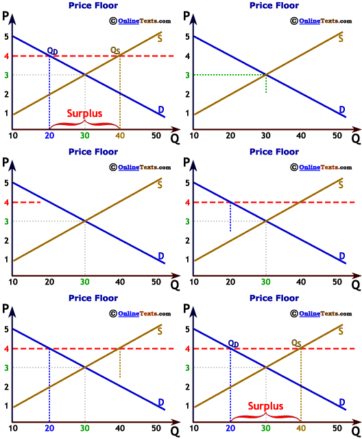
A price floor is a legal minimum that can be charged for a good.

Government Regulation of the Market: Price Ceilings and Floors

Sometimes the market equilibrium outcome is perceived by certain groups or individuals to be unfair or unjust. Societal values may dictate that the market outcome be altered. Government can intervene in markets in any number of ways, including the banning of the production and consumption of certain goods and services entirely. Government can also regulate heavily industries such as banking that it deems too sensitive to be left alone. We focus on two methods of government intervention: price ceilings and price floors.
A price ceiling specifies the legal maximum price

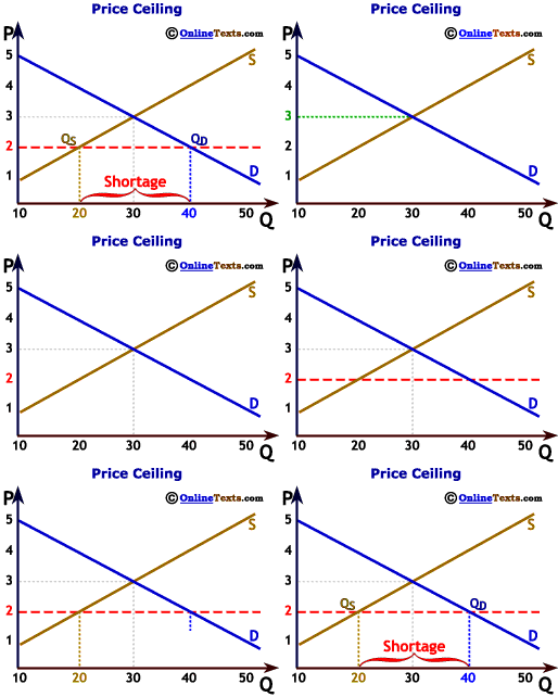
A price ceiling is a legal maximum that can be charged for a good. The ceiling is shown by a horizontal line at the ceiling price which--to be effective--is set below the equilibrium price. The figure titled "Price Ceiling" illustrates a ceiling at $2. At a price of $2 quantity demanded is 40 units and quantity supplied is 20 units. The result is a shortage in which quantity demanded exceeds quantity supplied.

Common examples of markets with price ceilings are apartment rentals and credit cards. Some municipalities such as Santa Monica, California impose maximum rents that can be charged for given apartments. For example, a ceiling of $1,000 per month might be set on two-bedroom apartments. In addition, some states have usury laws where interest rates are prevented from rising beyond a certain level. Credit card issuers in those states cannot charge interest rates above the ceiling.

Are these price ceiling justified? It depends. Equity is a subjective concept. Invariably, price ceilings help some groups and hurt others. For example, caps on apartment rents help tenants who pay below-market rents but hurt landlords and other prospective tenants who are shut out of the market due to the shortage. Santa Monica is plagued with buildings that landlords abandoned because the buildings became unprofitable to operate. Hence, the total supply of apartments in Santa Monica is lower than it otherwise would be.

Intervention in markets should not be taken lightly because often serious by-products emerge. With apartment price ceilings, underground markets often appear in which landlords and tenants agree to the "official" contract rate but tenants agree to make additional side payments. In addition, if landlords cannot set prices, they begin to adjust the quality of their apartments, letting them fall into disrepair. Some tenants end up living in unkempt conditions and are afraid to report the landlord because they may find themselves homeless if the landlord quits renting the apartment.

A price floor specifies the legal minimum price

A price floor is a legal minimum that can be charged for a good. The floor, as shown in the figure titled "Price Floor," is represented by a horizontal line. To be effective, the floor must be set above the equilibrium price. In the figure the floor is set at $4. Quantity demanded is 20 units and quantity supplied is 40 units. The result of the floor is a surplus of 20 units. Common examples of price floors are found in agricultural markets such as sugar, wheat and milk. The minimum wage is also a price floor because it sets a minimum dollar amount that employers can pay employees.

As with price ceilings, the same tradeoff occurs between equity and efficiency with price floors. Some groups benefit while others lose. In the case of the minimum wage, those who are able to find the higher paying jobs benefit. Employers who must pay higher wages lose along with those in the labor force who cannot find jobs because wages are too high. Agricultural price floors benefit farmers at the expense of consumers. Nevertheless, society has thus far deemed the benefits received from the price floors to be worth the costs.


Paradoxes Resolved

We now have the tools necessary to explain more fully some of the paradoxes presented at the beginning of the chapter. Why do school teachers earn $30,000 per year while some star athletes earn $18 million per year? Although differences in demand are important, the salary differentials are driven primarily by differences in the supply curves of the two markets. The number of excellent school teachers in the U.S. is quite high. To teach at most grade schools and high schools, one must attend college and typically earn a degree and an education certificate. Thousands of students take such a track in life. In contrast, star athletes are extremely rare. Home run hitters in baseball such as Babe Ruth, Mark McGwire and Barry Bonds only come along so often. Likewise, talented basketball players such as Michael Jordan and Moses Malone are rare. The incredibly small supply of such superstars, coupled with a high demand for their services, allows them to command enormous salaries. Is it fair that teachers are paid such dismal salaries relative to the athletes? Many teachers may not think so, but again, fairness is a relative concept.

A couple that purchases diamond engagement rings for one another are undoubtedly shocked by the high prices of diamonds. The same couple can stop at a water fountain and take drinks of water for free. Married couples can survive without diamond rings--water is essential. What accounts, then, for the high relative price for diamonds? Supply and demand factors both play important roles in this example. In most parts of the world, diamonds are in far shorter supply than drinking water. Consumers also value a diamond more than a glass of water under normal circumstances. The relatively small supply and the relatively high demand for diamonds drive their prices high relative to water.

Let's carry this paradox one step further. Suppose that the married couple somehow becomes stranded in the desert with no water to be found. A man approaches carrying a large jug of water. He offers to trade the water for the diamond rings. Does the couple make the exchange. Why or why not?


Copyright © 1996-2003 OnLineTexts.com, Inc. - All Rights Reserved